k-Means is a simple and popular unsupervised machine learning clustering algorithm, commonly used for market segmentation.
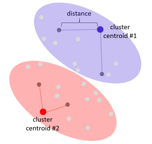
Assuming that there exists k number of clusters in a data set, the algorithm assigns each data point to the nearest cluster by computing the square of the distance between a data point and each cluster centroid. Based on these computations, a data point is assigned to a cluster centroid closest to it. At the beginning, the locations of the cluster centroids could be random. After each iteration, the algorithm moves each cluster centroid location to the computed arithmetic mean of all data points belonging to that cluster. Using the new cluster centroid locations, then recompute the squared distances for all the data points. The process iterates until each cluster centroid location stabilizes.
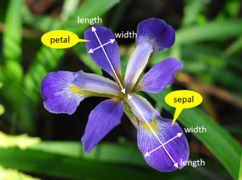
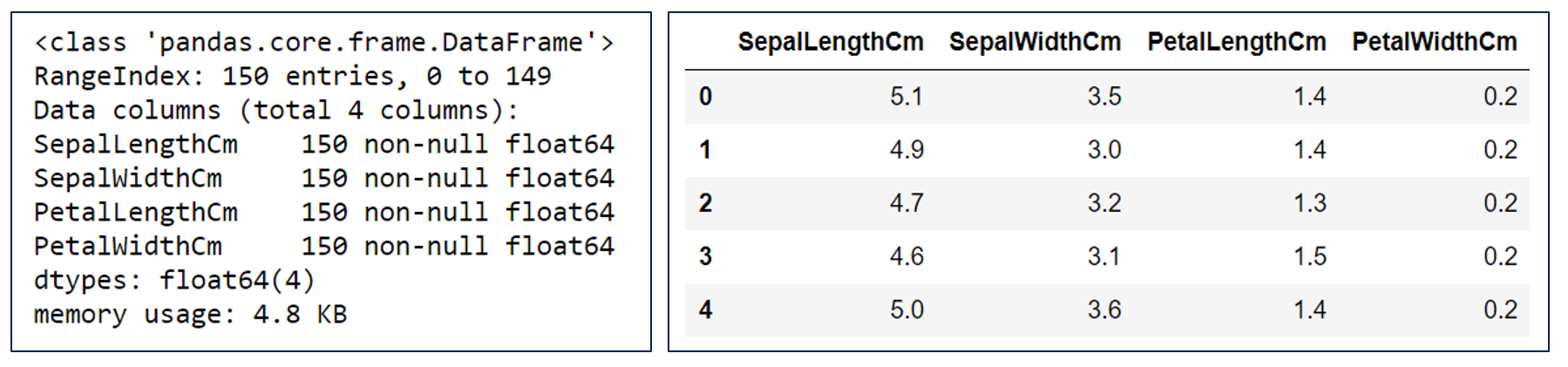
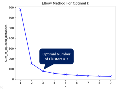
There is one problem though. How do we know how many clusters are there (i.e. what should be the value of k)? A common and simple solution is to use the Elbow method to determine the optimal number of clusters. To illustrate this approach, we will use the well documented multivariate Iris data set put together by the British statistician and biologist Robert Fisher in 1936. Fisher made meticulous measurements of the lengths and widths of the petals and sepals of 50 samples each of three Iris species – Setosa, Versicolor, Virginica. Each sample in the data set has 4 features (length of petal, width of petal, length of sepal, width of sepal) and a label (i.e. the species name).
Before using the Iris data set, we will remove all the labels (i.e. the species names) in Iris data set. k-Means is an unsupervised machine learning algorithm. There is no need for any labels in the data set.
Next, we will apply k-Means machine learning algorithm on this no-labels data set. We will compute and plot the sum of squared distances against the different values of k (starting from 1). The optimal number of clusters is given by the sharp turn in the Elbow graph. In this case, the optimal number is 3.
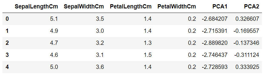
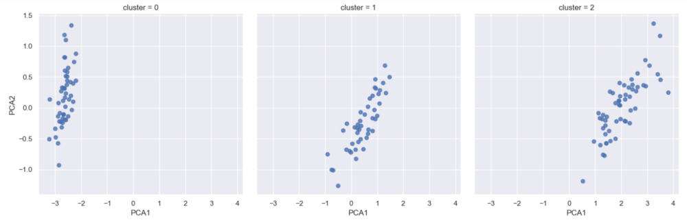
To verify that the optimal number is 3, we shall examine the cluster plots to see if they are distinct . Since it is almost impossible to visualize a 4-D graph (4 features) plot, let’s use the Principal of Component Analysis (PCA) technique to reduce the number of features to 2. Let’s call two reduced features PCA1 and PCA2.
Plotting the PCA2 against PCA1 for the 3 clusters show distinct plots, suggesting that there are 3 Iris species in the data set. Indeed, back in 1936 Robert Fisher had performed the petal and sepal measurements on exactly 3 species of Iris – Setosa, Versicolor and Virginica!
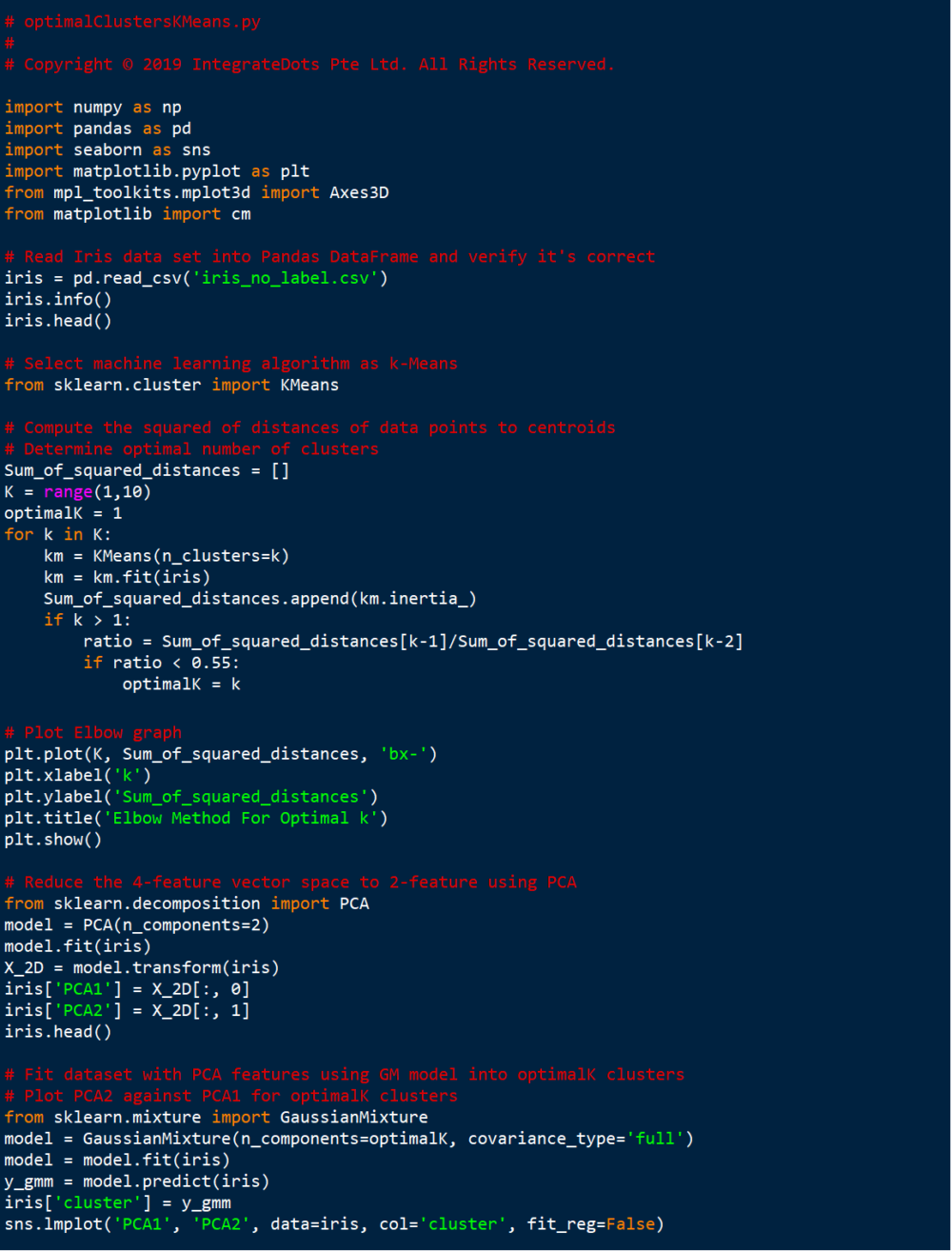
The Python code is shown below: